43 excel chart add data labels to all series
Chart.ApplyDataLabels method (Excel) | Microsoft Learn Applies data labels to all the series in a chart. Syntax expression. ApplyDataLabels ( Type, LegendKey, AutoText, HasLeaderLines, ShowSeriesName, ShowCategoryName, ShowValue, ShowPercentage, ShowBubbleSize, Separator) expression A variable that represents a Chart object. Parameters Example Data not showing on my chart [SOLVED] - Excel Help Forum May 03, 2005 · I'm sure it's something really stupid I overlooked - Charts are my weak area, but I've done several in the past just fine. I checked my source data three times now - - Each series name (from the row labels), and corresponding data for the series value is all accounted for. - Each column header shows in my category (X) axis.
Changing data label format for all series in a pivot chart Hi Shashaankmathur, To change data labels format, please perform the following steps: Click the pivot chart > + sign near tthe pivot chart > right click data label of any series > Format Data Series... Besides, to move forward, could you please provide the following information? 1. Do all series have data labels when you create a pivot chart?

Excel chart add data labels to all series
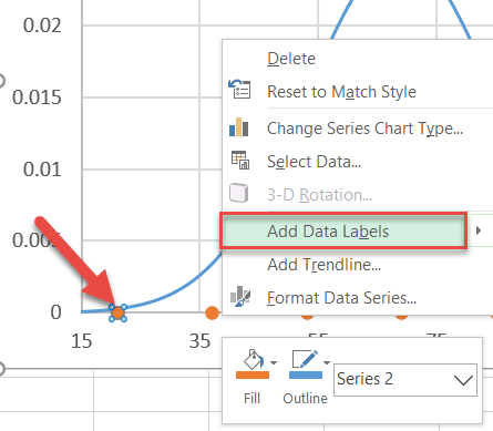
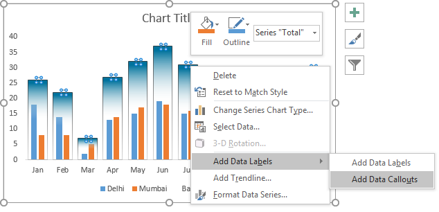
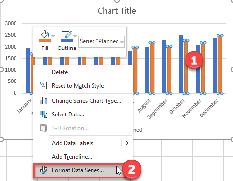
Trendlines and Chart Types in Excel - Peltier Tech So Excel uses 1 through 6 as X values, which match the Y values perfectly, resulting in a perfect fit to the formula y = x. The solution, of course, is to use an XY Scatter chart instead. X and Y values are all treated as numeric, and these numbers are used as is when calculating the trendline formula. The horizontal spacing of the points ... Excel Chart - Selecting and updating ALL data labels The following procedure accomplished your requirement; tell me how it works out for you: - Right-click a "point" in the series, which actually will be a bar piece. - Choose add data labels. - Right-click again and choose format data labels. - Check series name. - Uncheck value. Add or remove data labels in a chart - support.microsoft.com Click the data series or chart. To label one data point, after clicking the series, click that data point. In the upper right corner, next to the chart, click Add Chart Element > Data Labels. To change the location, click the arrow, and choose an option. If you want to show your data label inside a text bubble shape, click Data Callout.
Excel chart add data labels to all series. Excel Gantt Chart Tutorial + Free Template + Export to PPT Right-click the white chart space and click Select Data to bring up Excel's Select Data Source window. On the left side of Excel's Data Source window, you will see a table named Legend Entries (Series). Click on the Add button to bring up Excel's Edit Series window where you will begin adding the task data to your Gantt chart. Change the format of data labels in a chart To get there, after adding your data labels, select the data label to format, and then click Chart Elements > Data Labels > More Options. To go to the appropriate area, click one of the four icons ( Fill & Line, Effects, Size & Properties ( Layout & Properties in Outlook or Word), or Label Options) shown here. Series.DataLabels method (Excel) | Microsoft Learn This example sets the data labels for series one on Chart1 to show their key, assuming that their values are visible when the example runs. With Charts("Chart1").SeriesCollection(1) .HasDataLabels = True With .DataLabels .ShowLegendKey = True .Type = xlValue End With End With Support and feedback Formatting ALL data labels for ALL data series at once chart, go to the Chart menu > Chart Options > Data Labels tab. This does all series at once, not just the ones you've already labeled. You cannot apply other formatting to more than one series of labels at a time. - Jon J Jon Peltier Jan 18, 2008 #3 Ah yes. Excel 2007 has lost a lot of the familiar old dialogs. Since you're
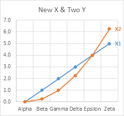
How to create waterfall chart in Excel - Ablebits.com Select your data including the column and row headers, exclude the Sales Flow column. Go to the Charts group on the INSERT tab. Click on the Insert Column Chart icon and choose Stacked Column from the drop-down list. The graph appears in the worksheet, but it hardly looks like a waterfall chart. Multiple Series in One Excel Chart - Peltier Tech Aug 09, 2016 · XY Scatter charts treat X values as numerical values, and each series can have its own independent X values. Line charts and their ilk treat X values as non-numeric labels, and all series in the chart use the same X labels. Change the range in the Axis Labels dialog, and all series in the chart now use the new X labels. How to add or move data labels in Excel chart? - ExtendOffice In Excel 2013 or 2016. 1. Click the chart to show the Chart Elements button . 2. Then click the Chart Elements, and check Data Labels, then you can click the arrow to choose an option about the data labels in the sub menu. See screenshot: In Excel 2010 or 2007. 1. click on the chart to show the Layout tab in the Chart Tools group. See ... Prevent Overlapping Data Labels in Excel Charts - Peltier Tech May 24, 2021 · In a line chart, all series use the same X values, so point 1 for all series is at the first X value, point 2 for all series is at the second X value, etc. This prevents my algorithm from being extended to XY charts with arbitrary, unsorted, and different X values for each series.
Chart elements Excel not showing - profitclaims.com A chart title will add a small textbox to the top of your chart allowing you to name/label it. You can expand the checkbox to reveal locations for the chart title to be created at: Data Labels. Data labels can be added to show a value or percentage to a chart that otherwise might be too difficult to read off the chart. How to set all data labels with Series Name at once in an Excel 2010 chart chart series data labels are set one series at a time. If you don't want to do it manually, you can use VBA. Something along the lines of. Sub setDataLabels() ' ' sets data labels in all charts ' Dim sr As Series Dim cht As ChartObject ' With ActiveSheet For Each cht In .ChartObjects For Each sr In cht.Chart.SeriesCollection sr.ApplyDataLabels ... Data Labels in Excel Pivot Chart (Detailed Analysis) Clicking on any Data labels one time will select all of the Data Labels simultaneously. Then right-click on the Data Table and from the context menu, click on the Format Data Labels. Then in the Format Data Labels, go to the Size and Properties. From there, click on the Text Directions. And from the drop-down menu, click on the Rotate all text 270. Excel Chart Tutorial: a Beginner's Step-By-Step Guide To do so, she’ll highlight all of the data (including column headers!) she wants included in her chart. Once her data is highlighted, she’ll head to the “Insert” menu in the ribbon and select what type of chart she wants to use to display her data. Excel offers tons of different types of charts to choose from, including: Line; Column ...
How to set all data labels with Series Name at once in an ...
How to add data labels in excel to graph or chart (Step-by-Step) Add data labels to a chart. 1. Select a data series or a graph. After picking the series, click the data point you want to label. 2. Click Add Chart Element Chart Elements button > Data Labels in the upper right corner, close to the chart. 3. Click the arrow and select an option to modify the location. 4.

How to Make Pie Chart with Labels both Inside and Outside ...
How to Add Total Data Labels to the Excel Stacked Bar Chart Apr 03, 2013 · Step 4: Right click your new line chart and select “Add Data Labels” Step 5: Right click your new data labels and format them so that their label position is “Above”; also make the labels bold and increase the font size. Step 6: Right click the line, select “Format Data Series”; in the Line Color menu, select “No line” Step 7 ...

Excel sunburst chart: Some labels missing - Stack Overflow
Dynamically Label Excel Chart Series Lines - My Online Training Hub Label Excel Chart Series Lines One option is to add the series name labels to the very last point in each line and then set the label position to 'right': But this approach is high maintenance to set up and maintain, because when you add new data you have to remove the labels and insert them again on the new last data points.

How to add data labels from different column in an Excel chart?
Add or remove data labels in a chart - support.microsoft.com Click the data series or chart. To label one data point, after clicking the series, click that data point. In the upper right corner, next to the chart, click Add Chart Element > Data Labels. To change the location, click the arrow, and choose an option. If you want to show your data label inside a text bubble shape, click Data Callout.

Adding rich data labels to charts in Excel 2013 | Microsoft ...
Excel Chart - Selecting and updating ALL data labels The following procedure accomplished your requirement; tell me how it works out for you: - Right-click a "point" in the series, which actually will be a bar piece. - Choose add data labels. - Right-click again and choose format data labels. - Check series name. - Uncheck value.
Multiple Series in One Excel Chart - Peltier Tech
Trendlines and Chart Types in Excel - Peltier Tech So Excel uses 1 through 6 as X values, which match the Y values perfectly, resulting in a perfect fit to the formula y = x. The solution, of course, is to use an XY Scatter chart instead. X and Y values are all treated as numeric, and these numbers are used as is when calculating the trendline formula. The horizontal spacing of the points ...

How to Add and Remove Chart Elements in Excel

Using the CONCAT function to create custom data labels for an ...

Directly Labeling Excel Charts - PolicyViz
insert-the-default-data-labels - Automate Excel

How to: Display and Format Data Labels | WPF Controls ...
Creative Column Chart that Includes Totals in Excel
Add Data Labels Outside End for Dynamic Label Threshold Chart ...
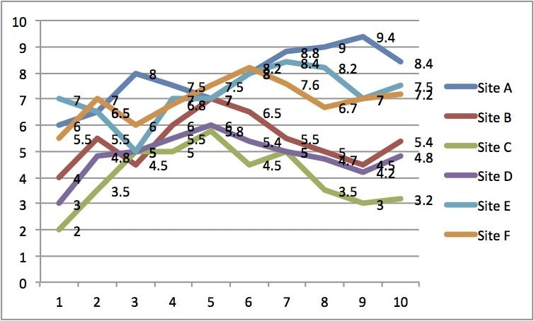
How to Create a Graph with Multiple Lines in Excel | Pryor ...

Total of chart series – Excel kitchenette

How to add data labels from different column in an Excel chart?

Custom data labels in a chart
How to Overlay Two Graphs in Excel – Automate Excel

Enable or Disable Excel Data Labels at the click of a button ...
Directly Labeling Excel Charts - PolicyViz

Chart Data Labels in PowerPoint 2013 for Windows

Adding rich data labels to charts in Excel 2013 | Microsoft ...

How to Add Data Labels to an Excel 2010 Chart - dummies

Add Total Values for Stacked Column and Stacked Bar Charts in ...

424 How to add data label to line chart in Excel 2016

How to use data labels in a chart

microsoft excel - Adding data label only to the last value ...

Add or remove data labels in a chart

How to Add Total Data Labels to the Excel Stacked Bar Chart ...
How to Place Labels Directly Through Your Line Graph in ...

Adding rich data labels to charts in Excel 2013 | Microsoft ...

Dynamically Label Excel Chart Series Lines • My Online ...

Adding rich data labels to charts in Excel 2013 | Microsoft ...

Google Workspace Updates: Get more control over chart data ...

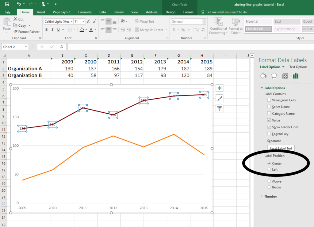
Change the format of data labels in a chart

Adding Data Labels to Your Chart (Microsoft Excel)
How to Create a Graph with Multiple Lines in Excel | Pryor ...

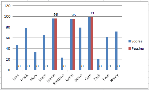
How to suppress 0 values in an Excel chart | TechRepublic

microsoft excel - Adding data label only to the last value ...

Excel charts: add title, customize chart axis, legend and ...
Move and Align Chart Titles, Labels, Legends with the Arrow ...

Add data labels and callouts to charts in Excel 365 ...

How to Add Total Data Labels to the Excel Stacked Bar Chart ...
Post a Comment for "43 excel chart add data labels to all series"