43 excel pivot table 2 row labels
Multiple row labels on one row in Pivot table | MrExcel Message Board I figured it out - Right click on your pivot table and choose pivot table options/display. Click on "Classic PivotTable layout" Then click on where it is subtotaling your row label and uncheck the subtotal option. D dudeshane0 New Member Joined Oct 23, 2014 Messages 1 Jan 19, 2015 #6 Gerald Higgins said: How to Concatenate Values of Pivot Table - Basic Excel Tutorial Click insert Pivot table, on the open window select the fields you want for your Pivot table. Once you select the desired fields, go to Analyze Menu. Under calculations, choose fields, Items & Sets tab then click on calculated fields. Enter the values and click ok. Your PivotTable will display the total of combined units and price.
› excel-pivot-table-formatHow to Format Excel Pivot Table - Contextures Excel Tips May 23, 2022 · Keep Formatting in Excel Pivot Table. A pivot table is automatically formatted with a default style when you create it, and you can select a different style later, or add your own formatting. For example, in the pivot table shown below, colour has been added to the subtotal rows, and column B is narrow.
Excel pivot table 2 row labels
Remove PivotTable Duplicate Row Labels - Excel Help Forum Re: Remove PivotTable Duplicate Row Labels Sometimes when the cells are stored in different formats within the same column in the raw data, they get duplicated. Also, if there is space/s at the beginning or at the end of these fields, when you filter them out they look the same, however, when you plot a Pivot Table, they appear as separate headers. Pivot Table "Row Labels" Header Frustration - Microsoft Tech Community Public Sector. Internet of Things (IoT) Azure Partner Community. Expand your Azure partner-to-partner network. Microsoft Tech Talks. Bringing IT Pros together through In-Person & Virtual events. MVP Award Program. Find out more about the Microsoft MVP Award Program. How to make row labels on same line in pivot table? Make row labels on same line with setting the layout form in pivot table As we all know, the pivot table has several layout form, the tabular form may help us to put the row labels next to each other. Please do as follows: 1. Click any cell in your pivot table, and the PivotTable Tools tab will be displayed. 2.
Excel pivot table 2 row labels. Combining two+ Columns to form one Row label column in Pivot Table Re: Combining two+ Columns to form one Row label column in Pivot Table Select a cell in your pivot table. Press Alt, then D, then P (i.e. in succession; not all at the same time), to call up the Pivot Table Wizard. Click "" button twice. Pivot table row labels in separate columns • AuditExcel.co.za Our preference is rather that the pivot tables are shown in tabular form (all columns separated and next to each other). You can do this by changing the report format. So when you click in the Pivot Table and click on the DESIGN tab one of the options is the Report Layout. Click on this and change it to Tabular form. Use column labels from an Excel table as the rows in a Pivot Table Highlight your current table, including the headers. Then from the Data section of the ribbon, select From Table. Highlight all the columns containing data, but not the Year column, and then select Unpivot Columns. Close the dialog and keep the changes. Excel should place the unpivoted data into a new worksheet, looking something like this: Design the layout and format of a PivotTable Click anywhere in the PivotTable. This displays the PivotTable Tools tab on the ribbon. On the Options tab, in the PivotTable group, click Options. In the PivotTable Options dialog box, click the Layout & Format tab, and then under Layout, select or clear the Merge and center cells with labels check box.
› excel-pivot-taHow to Create Excel Pivot Table [Includes practice file] Jan 15, 2022 · The area to the left results from your selections from [1] and [2]. You’ll see that the only difference I made in the last pivot table was to drag the AGE GROUP field underneath the PRECINCT field in the Row Labels quadrant. How to Create Excel Pivot Table. There are several ways to build a pivot table. get a row label from pivot table - Microsoft Tech Community @omdl2020 . GETPIVOTDATA() doesn't work in such case, it provides data if only it is visible in PivotTable. Alternatively you may work with cube assuming you are at least on Excel 2010, as I remember it's the first which supports data model. › blog › insert-blank-rows-inHow to Insert a Blank Row in Excel Pivot Table - MyExcelOnline Jan 17, 2021 · Pivot Table reports are shown in a Compact Layout format as a default and if you have two or more Items in the Row Labels (e.g.Month & Customer), then the Pivot Table report can look very clunky… There is a cool little trick that most Excel users do not know about that adds a blank row after each item, making the Pivot Table report look more ... en.wikipedia.org › wiki › Pivot_tablePivot table - Wikipedia Row labels are used to apply a filter to one or more rows that have to be shown in the pivot table. For instance, if the "Salesperson" field is dragged on this area then the other output table constructed will have values from the column "Salesperson", i.e. , one will have a number of rows equal to the number of "Sales Person".
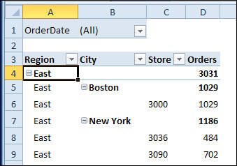
Pivot Table Row Labels In the Same Line - Beat Excel! First make a pivot table with required fields. Arrange the fields as shown in left picture. Your initial table will look like right picture. Now click on "Error Code" and access field settings. First check "None" option in "Subtotals & Filters" tab to disable totals after every row. Excel Pivot Table Row labels - Stack Overflow 1 Answer. Sorted by: 0. Right click on the pivot, go to PivotTable Options, Display Tab. Click on "Classic Pivot Table Layout". Go to each field (column), right click, field settings, layout & print tab. Click on "Repeat Item Labels". That should give you the table you're looking for. How to rename group or row labels in Excel PivotTable? 1. Click at the PivotTable, then click Analyze tab and go to the Active Field textbox. 2. Now in the Active Field textbox, the active field name is displayed, you can change it in the textbox. You can change other Row Labels name by clicking the relative fields in the PivotTable, then rename it in the Active Field textbox. Multi-level Pivot Table in Excel (In Easy Steps) First, insert a pivot table. Next, drag the following fields to the different areas. 1. Order ID to the Rows area. 2. Amount field to the Values area. 3. Country field and Product field to the Filters area. 4. Next, select United Kingdom from the first filter drop-down and Broccoli from the second filter drop-down.
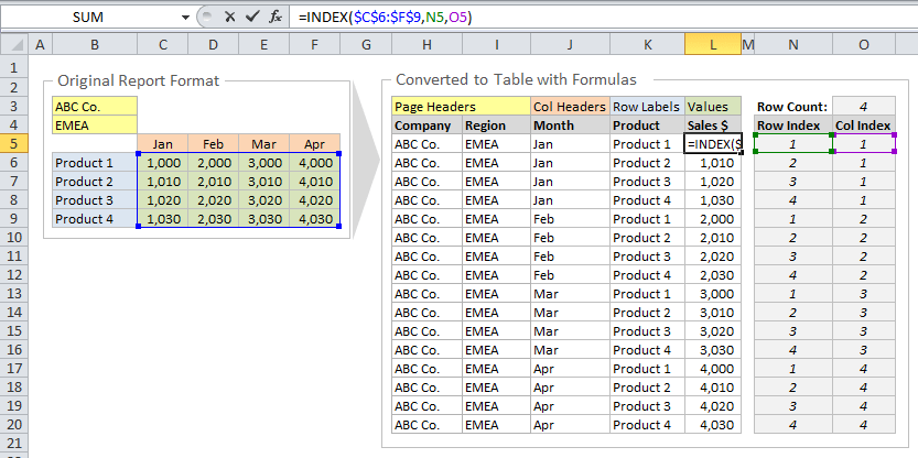
How to Setup Source Data for Pivot Tables - Unpivot in Excel
Pivot table-Displaying multiple Row Labels on one line Without knowing how your data is setup, its hard to know how the pivot is responding to your data. First though, set your pivot table in classic view. To do this, go to Pivot Table Options>Display>Select Classic Pivot Table Layout. Then put your region and address in the Row Labels section. See how that works.

How to group by range in an Excel Pivot Table?
Automatic Row And Column Pivot Table Labels - How To Excel At Excel Select the data set you want to use for your table The first thing to do is put your cursor somewhere in your data list Select the Insert Tab Hit Pivot Table icon Next select Pivot Table option Select a table or range option Select to put your Table on a New Worksheet or on the current one, for this tutorial select the first option Click Ok

How to Sort Data in a Pivot Table | Excelchat
Pivot Table Two Row Labels Excel - how-use-excel.com Pivot Table Two Row Labels Excel Excel Details: Except repeating the row labels for the entire pivot table, you can also apply the feature to a specific field in the pivot table only. 1. Firstly, you need to expand the row labels as outline form as above steps shows, and click one row label which you want to repeat in your pivot table. 2.
Repeat Pivot Table Labels in Excel 2010 - Excel Pivot TablesExcel Pivot Tables
multiple fields as row labels on the same level in pivot table Excel ... multiple fields as row labels on the same level in pivot table Excel 2016 I am using Excel 2016. I have data that lists product models along with relevant data and also production volumes by month. Part of the relevant data are about 5 common part columns with the part # that applies to each model under the appropriate column.

How to Sort Pivot Table Row Labels, Column Field Labels and Data Values with Excel VBA Macro ...
Repeat item labels in a PivotTable - support.microsoft.com Right-click the row or column label you want to repeat, and click Field Settings. Click the Layout & Print tab, and check the Repeat item labels box. Make sure Show item labels in tabular form is selected. Notes: When you edit any of the repeated labels, the changes you make are applied to all other cells with the same label.

Excel Pivot Table Report - Sort Data in Row & Column Labels & in Values Area, use Custom Lists
Pivot table row labels side by side - Excel Tutorials You can copy the following table and paste it into your worksheet as Match Destination Formatting. Now, let's create a pivot table ( Insert >> Tables >> Pivot Table) and check all the values in Pivot Table Fields. Fields should look like this. Right-click inside a pivot table and choose PivotTable Options…. Check data as shown on the image below.

Rename Pivot Table Row Labels | Decorations I Can Make
powerspreadsheets.com › excel-pivot-table-groupExcel Pivot Table Group: Step-By-Step Tutorial To Group Or ... In fact, as mentioned in Excel 2016 Pivot Table Data Crunching: Each time you create a new pivot table in Excel 2016, Excel automatically shares the pivot cache. Pivot Cache sharing has several benefits. Most notably, as I mention above, it reduces memory requirements and file size vs. the scenario where the Pivot Cache isn't shared.

How to Sort Pivot Table Row Labels, Column Field Labels and Data Values with Excel VBA Macro ...
blog.hubspot.com › marketing › how-to-create-pivotHow to Create a Pivot Table in Excel: A Step-by-Step Tutorial Dec 31, 2021 · After you've completed Step 3, Excel will create a blank pivot table for you. Your next step is to drag and drop a field — labeled according to the names of the columns in your spreadsheet — into the Row Labels area. This will determine what unique identifier — blog post title, product name, and so on — the pivot table will organize ...

Excel pivot table categorical variables the same in multiple columns (histogram) - Super User
excel - Incorrect Calculations in Pivot table when adding a measure ... Incorrect Calculations in Pivot table when adding a measure. I have made a pivot table of data in which there is a row label and two columns - sum of amount and sum of the actual cost of units, also I have added a measure (profit) which has the formula of subtraction between two sums column. After adding the profit measure to the pivot table ...

Pivot Table Multiple Row Labels Side By Side
How to Customize Your Excel Pivot Chart Data Labels - dummies The Data Labels command on the Design tab's Add Chart Element menu in Excel allows you to label data markers with values from your pivot table. When you click the command button, Excel displays a menu with commands corresponding to locations for the data labels: None, Center, Left, Right, Above, and Below. None signifies that no data labels ...

Turn off automatic date and time grouping in Excel Pivot Tables
› excel-pivot-table-subtotalsExcel Pivot Table Subtotals - Contextures Excel Tips Feb 01, 2022 · In the pivot table shown below, Service is in the Row Labels area, Lead Tech is in the Column Labels area, and Labor Cost is in the Values area. Because Service is the only field in the Row Labels area, it has no subtotal. Multiple Row Fields. When you add another field to the Row Labels area, a subtotal is automatically created for the first ...

Create a pie chart from distinct values in one column by grouping data in Excel - Super User
Pivot Table adding "2" to value in answer set 1) Right click your pivot table -> Pivot table options -> Data -> Change "Number of items to retain per field" to NONE 2) Wipe all rows in your data source except for the headers 3) Refresh the pivot table 4) Save, and close all instances of Excel 5) Reopen the file, and paste your data 6) Refresh the pivot table

vba - Displaying rows based on column label in Excel for a Pivot Table - Stack Overflow
How to repeat row labels for group in pivot table? - ExtendOffice In Excel, when you create a pivot table, the row labels are displayed as a compact layout, all the headings are listed in one column. Sometimes, you need to convert the compact layout to outline form to make the table more clearly. But in tphe outline layout, the headings will be displayed at the top of the group.

How to Show the Percentage of Row Total in the Pivot Table - MS Excel | Excel In Excel
Formula1, Formula2 appearing as row items in pivot table where row ... if you select a row item and go to the botttom right of the cell to the black cross hairs and drag down, it inserts formula1, formula2 formula3 depend how far you dragged it, and the appear in multiple cells in the pivot table. The solution is as listed above. Going to pivot table, Analyse, Fields, items & sets, solve order and deleting the ...

Excel Help: Simple method to make Pivot table
How to make row labels on same line in pivot table? Make row labels on same line with setting the layout form in pivot table As we all know, the pivot table has several layout form, the tabular form may help us to put the row labels next to each other. Please do as follows: 1. Click any cell in your pivot table, and the PivotTable Tools tab will be displayed. 2.
Post a Comment for "43 excel pivot table 2 row labels"